Dissipative Ising Model

By Dawid Hryniuk, Jack Dunham

In this tutorial, we will use exact diagonalization, VMPOMC.jl and t-VMPOMC.jl to study the properties of a class of dissipative transverse-field Ising models.

Recommended tutorials

Julia

Introduction

We consider a transverse-field Ising model in one-dimension described by the Hamiltonian \begin{equation} H = J\sum_i \sigma^z_i \sigma^z_{i+1} + h\sum_i \sigma^x_i. \end{equation} The ground state properties of the system are well understood. Here, we are interested in exploring its non-equilibrium properties. We assume that the interactions of the system of spins with the external enviornment is well described by a Markovian Lindblad master equation for the many-body density matrix $\rho$, \begin{equation} \partial_t \rho = -i[H,\rho] + \sum_k \left(\Gamma_k \rho \Gamma_k^\dagger - \frac{1}{2}{\Gamma_k^\dagger \Gamma_k,\rho}\right) := \mathcal{L}[\rho] \end{equation} The superoperator $\mathcal{L}$ is often referred to as the Lindbladian. Here, each jump operator $\Gamma_k$ encodes a specific dissipative process acting on site $k$. In this example we choose \begin{equation} \Gamma_k = \sqrt{\gamma}\,\sigma^-_k, \end{equation} where

• $\sigma^- = (\sigma^x - i\sigma^y)/2$ is the spin-lowering operator on a single site.
• $\gamma$ is the dissipation rate (we set $\gamma=1$ in our units).

Physically, $\Gamma_k$ implements spontaneous emission of an excited spin into the environment, driving each spin toward the $|\downarrow\rangle$ state. The competition among the interaction between neighbouring spins ($J\sigma^z_i\sigma^z_{i+1}$), coherent transverse-field flips ($h\sigma^x$) and dissipative decay ($\sqrt{\gamma}\sigma^-$) gives rise to nontrivial non-equilibrium dynamics and steady states. Other common choices include:

• Dephasing: $\Gamma_k = \sqrt{\gamma_z}\sigma^z_k$, which randomizes the relative phase in the $[\ket{\uparrow}, \ket{\downarrow}]$ basis without changing populations.
• Collective decay: $\Gamma = \sqrt{\gamma_c},\sum_k \sigma^-_k$, coupling the entire chain to a common bath and leading to superradiant effects.

Steady state

We will begin by investigating the non-equilibrium steady state of the model, i.e. the fixed point of the dynamics reached at very long times, $\partial_t \rho = 0$. We will do so with the help of exact diagonalization and the time-independent variational principle.

Exact diagonalization

Let us begin by constructing and diagonalizing the Lindbladian superoperator. We first load the necessary packages and define Pauli operators, along with their sparse variants:

using LinearAlgebra, SparseArrays, ArnoldiMethod

⊗(x,y) = kron(x,y)

id = [1.0+0.0im 0.0+0.0im; 0.0+0.0im 1.0+0.0im]
sx = [0.0+0.0im 1.0+0.0im; 1.0+0.0im 0.0+0.0im]
sy = [0.0+0.0im 0.0-1im; 0.0+1im 0.0+0.0im]
sz = [1.0+0.0im 0.0+0.0im; 0.0+0.0im -1.0+0.0im]
sp = (sx+1im*sy)/2
sm = (sx-1im*sy)/2

sp_id = sparse(id)
sp_sx = sparse(sx)
sp_sy = sparse(sy)
sp_sz = sparse(sz)
sp_sp = sparse(sp)
sp_sm = sparse(sm)

We then construct the Ising Hamiltonian:

function one_body_Hamiltonian_term(N::Int64, op::SparseMatrixCSC{ComplexF64, Int64})
    ops = fill(sp_id, N)
    ops[1] = op
    H = spzeros(ComplexF64, 2^N, 2^N)
    for _ in 1:N
        H += foldl(⊗, ops)
        ops = circshift(ops,1)
    end
    return H
end

function two_body_Hamiltonian_term(N::Int64, op::SparseMatrixCSC{ComplexF64, Int64})
    ops = fill(sp_id, N)
    ops[1] = op
    ops[2] = op
    H = spzeros(ComplexF64, 2^N, 2^N)
    for _ in 1:N
        H += foldl(⊗, ops)
        ops = circshift(ops,1)
    end
    return H
end


N = 8
J = 0.5
h = 1.0

H = J * two_body_Hamiltonian_term(N, sp_sz) + h * one_body_Hamiltonian_term(N, sp_sx)

The Lindbladian can be expressed as a matrix in Liouville space. The (non-unique) isomorphism is given by \begin{align} \mathcal{L} &= -i( H\otimes \mathbb{1} - \mathbb{1} \otimes H^\top ) + \sum_k \left(\Gamma_k \otimes \Gamma_k^* - \frac{1}{2}\Gamma_k^\dagger \Gamma_k \otimes \mathbb{1} - \frac{1}{2} \mathbb{1} \otimes \Gamma_k^\top \Gamma_k^* \right). \end{align} In Julia:

function one_body_Lindbladian_term(N::Int64, op::SparseMatrixCSC{ComplexF64, Int64})
    ops = fill(sp_id, N)
    ops[1] = op
    Id = foldl(⊗, fill(sp_id, N))
    L_D = spzeros(ComplexF64, 2^(2*N), 2^(2*N))
    for _ in 1:N
        Γ = foldl(⊗, ops)
        ops = circshift(ops,1)
        L_D += Γ⊗conj(Γ) - (conj(transpose(Γ))*Γ)⊗Id/2 - Id⊗(transpose(Γ)*conj(Γ))/2
    end
    return L_D
end

γ = 1.0
Id = foldl(⊗, fill(sp_id, N))
L = -1im*(H⊗Id - Id⊗transpose(H)) + γ * one_body_Lindbladian_term(N, sp_sm)

L is now a sparse, non-Hermitian, square matrix, which can be diagonalized via the Arnoldi method. We write:

function eigen_sparse(x, n)
    decomp, history = partialschur(x, nev=n, which=:LR, restarts=100000);
    vals, vecs = partialeigen(decomp);
    return vals, vecs
end

evals, evecs = eigen_sparse(L, 6)

display(evals)

This finds the 6 largest eigenvalues, which are found to be all non-positive, with one zero eigenvalue associated with the unique steady state:

6-element Vector{ComplexF64}:
     -1.0265353581717023 - 3.36845317347161e-11im
     -1.0258847238574662 - 4.232719954352772e-10im
     -1.0174169414337269 + 2.594555839820057im
      -1.017416941284772 - 2.594555839810845im
     -0.5105598311206574 + 4.4948856307595167e-10im
 -3.1922988069600096e-10 + 9.084818965830727e-11im

The eigenvector associated with the zero eigenvalues can be reshaped and renormalized to obtain the steady-state density matrix:

ρ = reshape(evecs[:,end] ,2^N, 2^N)
ρ./=tr(ρ)
display(ρ)

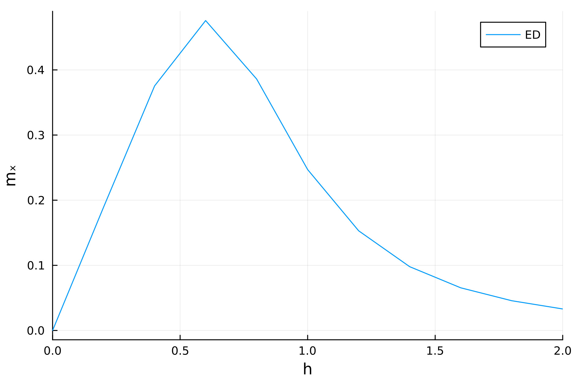
One can then, for example, study the steady-state magnetization phase diagram as function of the transverse field strength $h$, given by $m_x = \text{tr}\, {\sigma^x\rho}$. This can be achieved via

function magnetization(op, site::Int64, ρ::Matrix{ComplexF64}, N::Int64)
    first_term_ops = fill(id, N)
    first_term_ops[site] = op
    m = tr(ρ*foldl(⊗, first_term_ops))
    return m
end

mx_list = []
h_range = 0.0:0.2:2.0
for h=h_range
    H = J * two_body_Hamiltonian_term(N, sp_sz) + h * one_body_Hamiltonian_term(N, sp_sx)
    L = -1im*(H⊗Id - Id⊗transpose(H)) + γ * one_body_Lindbladian_term(N, sp_sm)
    evals, evecs = eigen_sparse(L, 2)
    ρ = reshape(evecs[:,end],2^N,2^N)
    ρ./=tr(ρ)
    mx = magnetization(sx, 1, ρ, N)
    push!(mx_list, real(mx))
end

using Plots

plot(h_range, mx_list, xlims=(0,2), xlabel="h", ylabel="mₓ")

This produces the below figure:

VMPOMC

Exact diagonalization of the Liouvillian scales exponentially in system size and quickly becomes intractable. To reach $N=20$ spins, we employ the variational matrix product operator Monte Carlo (VMPOMC) method, which approximates the steady-state density operator $\rho_{ss}$ as a parameterized MPO and optimizes it stochastically. Below is a minimal script:

include("VMPOMC.jl")
using .VMPOMC
using LinearAlgebra
using MPI


MPI.Init()
mpi_cache = set_mpi()

N = parse(Int64, ARGS[1])
h = parse(Float64, ARGS[2])
χ = parse(Int64, ARGS[3])

# Physical parameters
const J = 0.5
const γ = 1.0

# Optimization hyperparameters
const N_MC = 250
const δ = 0.1
const F = 0.998
const ϵ = 0.1
const N_iterations = 5000
const cost_function_threshold = 1e-4

# Initialize parameters (use positional arguments)
params = Parameters(N=N, χ=χ, J=J, hx=h, γ=γ)

# Define the one-body Lindbladian:
l1 = make_one_body_Lindbladian(h*sx, sqrt(γ)*sm)

# Initialize MPO on all processes
A = Array{ComplexF64}(undef, χ, χ, 4)

if mpi_cache.rank == 0
    A_init = rand(ComplexF64, χ, χ, 2, 2)
    A = reshape(A_init, χ, χ, 4)
end
MPI.Bcast!(A, 0, mpi_cache.comm)

# Define sampler and optimizer
sampler = MetropolisSampler(N_MC, 2)
optimizer = Optimizer("SR", sampler, A, l1, ϵ, params, "Ising", "Local")

# Variable to track convergence
converged = false

for k in 1:N_iterations
    # Optimize MPO
    compute_gradient!(optimizer)
    MPI_mean!(optimizer, mpi_cache)
    
    if mpi_cache.rank == 0
        optimize!(optimizer, δ*F^k)
    end
    
    MPI.Bcast!(optimizer.A, 0, mpi_cache.comm)
    
    if mpi_cache.rank == 0
        # Calculate energy per site
        cost_function = real(optimizer.optimizer_cache.mlL)/N
        
        # Check for convergence (cost_function below threshold)
        if abs(cost_function) < cost_function_threshold
            global converged = true
        end
        
        # Print progress every 100 iterations or on final iteration
        if mod(k, 100) == 0 || converged
            # Calculate steady-state magnetizations
            mx = tensor_calculate_magnetization(optimizer, sx)

            println("Iteration $k:")
            println("  Cost Function: $(round(cost_function, digits=6))")
            println("  Magnetization: mx=$(round(mx, digits=4))")
        end
    end
    
    # Broadcast convergence status to all processes
    MPI.bcast(converged, mpi_cache.comm)
    
    # Exit loop if converged
    if converged
        break
    end
end

if mpi_cache.rank == 0
    if converged
        # Record magnetization
        mx = tensor_calculate_magnetization(optimizer, sx)
        o = open("Ising_h=$(h)_mx.txt", "a")
        println(o, real(mx))
        close(o)
        println("Optimization completed successfully with convergence!")
    else
        println("Optimization completed - maximum iterations reached without convergence.")
        energy = real(optimizer.optimizer_cache.mlL)/N
        println("Final Cost Function: $(round(energy, digits=8))")
    end
end

MPI.Finalize()
exit(0)

This script can be ran by executing

mpirun -np X julia vmpomc_ising.jl N h chi

where X specifies the number of MPI processes, N is the number of sites, h is the local field strength, and chi is the bond dimension.

Note on hyperparameters:
The above script makes use of five hyperparameters that control the gradient descent optimization:

• N_MC: Number of Monte Carlo samples used in the Metropolis sampler. Increasing this improves sampling accuracy but increases computational cost.
• δ: Initial learning rate scaling factor for the optimizer.
• F: Learning rate decay factor per iteration, controlling how the learning rate decreases over time.
• ϵ: Regularization parameter used in the optimizer to stabilize the inversion of the metric matrix. Effectively tunes between SGD and SR.
• N_iterations: Maximum number of optimization iterations.
• cost_function_threshold: Threshold for the cost function below which optimization is considered converged. Ideally, we want this to be as close to 0 as possible.

Adjusting these parameters affects convergence speed and stability. Start with the above pre-set defaults and tune based on problem size, bond dimension, and observed convergence behavior.

To reproduce the phase diagram as in ED, we can run the bash script:

#!/bin/bash

N=20
CHI=6

for i in $(seq 2 8); do
    h=$(echo "scale=1; $i / 5.0" | bc)
    echo "Running h = $h"
    mpirun -np 4 julia vmpomc_ising.jl $N $h $CHI
done

echo "Done"

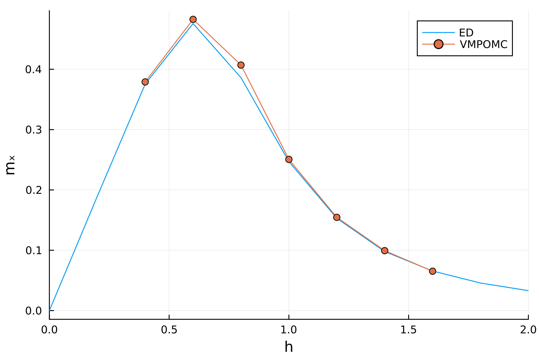
The converged magnetizations for $N=20$ can now be loaded and plotted against ED results for $N=8$, showing excellent agreement:

Exercises

• A bond dimension of $χ=6$ is found to give accurate estimates of the magnetization at low computational overhead at $N=20$, but larger χ improves fidelity at increased cost. To see this, fix the value of the local field $h$ and plot the converged magnetizations as function of the bond dimension, starting from $χ=1$, tracking the attained values of the cost function. Use the time() function in Julia to also track the total optimization time. Observe how an insufficiently small bond dimension causes the cost function to plateau at a value that may higher than the set threshold, preventing the results from ever converging.
• What happens when we increase or decrease the interaction strength $J$? What is the minimum bond dimension required for convergence in those cases?
• Try to vary and find the optimal hyperparameter values that lead to most rapid convergence. How much can the convergence threshold be loosened before the results become inaccurate?
• Suppose the interaction with the external environment leads to spin decay to the $\ket{\rightarrow}$ state, described by the Lindblad jump operator $\Gamma_k = \sqrt{\gamma}(\sigma^z - i\sigma^y)/2$. Compare the resultant phase diagrams for $m_x$, $m_y$, and $m_z$.
• Instead of starting each optimization process from a completely random MPO, it may be more efficient to load an already converged MPO at slightly different model parameter values. Try implementing this by appropriately modifying the above scripts.

Two-dimensional lattices - iPEPO

We will now consider the two-dimensional dissipative Ising model. To do so, we will use a two-dimensional tensor network ansatz known as an infinite projected-entangled pair state to solve the dissipative Ising model directly in the thermodynamic limit. To get started, load TimeEvolutionPEPO.jl and the TensorKit package.jl

using TimeEvolutionPEPO
using TensorKit

Computing Observables

To calculate expectation values of observables, one must first construct a reduced density matrix from the tensor network. To do this, a boundary algorithm (and associated boundary bond dimension) must be chosen to compute the partial trace of the environment around those lattice sites to be left untraced. Such an object is represented by the DensityMatrix struct found in the TimeEvolutionPEPO package. A DensityMatrix can the be used to compute reduced density matrices.

function magnetisation(pepo::PEPO; alg = CTMRG(bonddim = 16, tol = 1e-8, verbose=false))
    dm = DensityMatrix(pepo, alg)
    rdm = partialtrace(dm, (1,1))

    M = expval(rdm, PAULI[1])

    return real(M)
end

In practice it is useful to save the DensityMatrix object rather than running the boundary renormalization every time one wishes to compute a local observable. Also, the correlation length of a state can be directly accessed directly from the DensityMatrix object without first needing to compute a partial trace:

Running the Simulation

Simulations must first be initialised using three arguments. First, a tensor network representation of an initial state must be defined. This can be one obtained from a different Simulation object by calling the function quantumstate on this object to return the PEPO associated with that simulation.

function newsim(model)
    # Set initial state to a product state of spins pointing down along the z-axis on a two-by-two
    # unit-cell
    ρ = fill((0,0,-1), 2, 2)

    # Set the bond dimension equal to 4
    D = 4

    # Initialise using the TEBD (with default options)
    method = TEBD()

    # Construct the tensor network. 
    state = PEPO(ρ, 4)

    sim = Simulation(state, model, method; timestep=0.025)

    return sim
end

We can then run the simulation be calling simulate!.

function runsim!(sim)
    magn = Float64[]
    time = Float64[]

    # This custom function is executed at regular intervals during the simulation
    callback = sim -> begin
        # Get some useful simulation information 
        info = simulationinfo(sim)

        # Get tge `PEPO` object contained in `sim`
        state = quantumstate(sim)

        push!(magn, magnetisation(state))
        push!(time, info.simtime)
    end

    # Initially, dynamics are faster, so execute callback every time step
    simulate!(callback, sim; numsteps = 50, maxshots = 50, verbose=false)

    # Sample only every 3rd time step for another 150 steps
    simulate!(callback, sim; numsteps = 150, maxshots = 50, verbose=false)

    return magn, time
end

This time we will consider a different Ising model from the one used in the previous part of this tutorial, namely one with a transverse dissipator (along the $x$-axis) admitting an exact solution in the thermodynamic limit. Mathematically, the Hamiltonian is the following: \begin{equation} H = \frac{J}{4} \sum_{\langle i,j \rangle} \sigma^{z}_i \sigma^{z}_j \end{equation} with transverse dissipation $\Gamma_j = \frac{\sqrt{\gamma}}{2}(\sigma^y_j - i\sigma^z_j)$ which can be constructed in the TimeEvolutionPEPO package like so:

X, Y, Z = PAULI
model = J -> Model(J / 4 * LocalOp(Z,Z) + Dissipator(0.5 * (Y - im * Z)))

where again we have set $\gamma = 1$. This can then be passed into the functions we have defined previously.

sim = newsim(model(1.0, 0.5));
magn, time = runsim!(sim);

Note the Simulation object sim mutates in the process. Some information pertaining to a given Simulation object can be obtained by calling:

simulationinfo(sim)

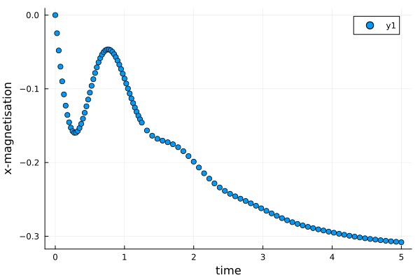
which can also be accessed in the callback function. Lets plot the results of the simulation using the Plots.jl package.

using Plots.jl # Make sure this is `add`ed to you environment!
scatter(time, magn; xlabel = "time", ylabel = "x-magnetisation")

Exact Solution

This model can be solved exactly with help from the QuantumOptics package:

using QuantumOptics

function ising_transverse_dissipator(J)
    # Hamiltonian
    basis = SpinBasis(1 // 2)
    Id = identityoperator(basis)

    σz = sigmaz(basis)

    Γ = 0.5 * (sigmaz(basis) - im * sigmay(basis))

    ⊗ = QuantumOptics.:⊗
    H = J / 4 * σz ⊗ σz ⊗ Id ⊗ Id ⊗ Id
    H += J / 4 * σz ⊗ Id ⊗ σz ⊗ Id ⊗ Id
    H += J / 4 * σz ⊗ Id ⊗ Id ⊗ σz ⊗ Id
    H += J / 4 * σz ⊗ Id ⊗ Id ⊗ Id ⊗ σz

    Id = one(Γ)

    Idlist = [Id for i in 1:5]
    Idlist[1] = Γ
    L = [tensor(circshift(Idlist, n)...) for n in 0:4]

    return H, L
end

function exactsolve(J; numshots = 101, tf = 5.0)
    ⊗ = QuantumOptics.:⊗

    time = collect(range(0.0, tf, numshots))

    basis = SpinBasis(1 // 2)

    Ψzd = spindown(basis)

    ρn = QuantumOptics.:⊗(Ψzd, dagger(Ψzd))
    ρ0 = tensor([ρn for site in 1:5]...)

    Id = identityoperator(basis)
    σx = sigmax(basis)

    H, L = ising_transverse_dissipator(J)

    _, ρ_time_master = timeevolution.master(time, ρ0, H, L)

    sx_time = real(QuantumOptics.expect(σx ⊗ Id ⊗ Id ⊗ Id ⊗ Id, ρ_time_master))
    return time, sx_time
end

Exercises

• Compare the results from the simulation to the exact solution. What do you think the source of the discrepancy is?
• Consider both reducing the time step and increasing the bond dimension of the iPEPO ansatz. Are you able to obtain results visually indistinguishable from the exact solution? What about if you increasing the strength of the interaction $J$?
• By default, the TEBD algorithm in TimeEvolutionPEPO uses the simple update method to truncate each bond at each time step and therefore does not take into account the full lattice during truncation. Do you expect this to lead to significant truncation errors in general? Why or why not?
• Consider the previous question in the context of the exactly solvable model studied here. Do you have some intuition as to why such a model is so amenable to simulations using simple update?
• Try introducing a transverse field. How does this effect the performance of the simulation?