Driven Dissipative Bose-Hubbard Model

By Alex Ferrier

In this tutorial, we will use Positive P to study the behaviour of some examples of driven dissipative Bose-Hubbard (DDBH) models.

Recommended tutorials

xmds2

Introduction

In the most general form, without at this stage specifying the lattice geometry, the Hamiltonian for a driven Bose-Hubbard (DDBH) model can be written in the frame rotating with the driving frequency as

\[\hat{H} = \sum_j \left( -\Delta\hat{a}^\dagger_j\hat{a}_j +\frac{U}{2}\hat{a}^\dagger_j\hat{a}^\dagger_j\hat{a}_j\hat{a}_j +F_j\hat{a}^\dagger_j + F_j^*\hat{a}_j \right) -\sum_{j,j'} \left(J_{j,j'}\hat{a}^\dagger_j\hat{a}_{j'} + J^*_{j,j'}\hat{a}^\dagger_{j'}\hat{a}_j \right) \, ,\]

where $\Delta$ gives the detuning between the on-site energy and the driving frequency, $U$ the two-body interaction strength, $F_j$ the driving amplitude on each site $j$, and $J_{j,j’}$ the hopping between sites (typically $J_{j,j’} = J$ for connected sites and 0 otherwise). Including the effects of dissipation to the external environment, the evolution of the system as described by the many-body density matrix $\hat{\rho}$ is given by a Markovian Lindblad master equation

\begin{equation} \frac{\partial\hat{\rho}}{\partial t} = -i\left[\hat{H}, \hat{\rho}\right] + \sum_j\frac{\gamma}{2}\left(2\hat{a}_j\hat{\rho}\hat{a}^\dagger_j - \hat{a}^\dagger_j\hat{a}_j\hat{\rho} - \hat{\rho}\hat{a}^\dagger_j\hat{a}_j\right) \, , \end{equation}

where $\gamma$ is the dissipation rate (we set $\gamma=1$ in our units).

Single Site

Positive-P method

We will start by calculating the observables for the limiting case of the model of a single site nonlinear bosonic mode with consequently no hopping term. Using Positive-P simulations, we generate sets of stochastic trajectories for two complex variables $\alpha(t)$ and $\beta(t)$. We will calculate the occupation $n$ and second-order correlation $g^{(2)}(0)$, which in the positive-P representation can be calculated by corresponding averages over trajectories:

\[n = \langle \hat{a}^\dagger \hat{a} \rangle = \langle \alpha \beta \rangle_{PP}\, ,\] \[g^{(2)}(0) = \frac{\langle \hat{a}^\dagger \hat{a}^\dagger \hat{a} \hat{a} \rangle}{\langle \hat{a}^\dagger \hat{a} \rangle^2} = \frac{\langle \alpha^2 \beta^2 \rangle_{PP}}{\langle \alpha \beta \rangle_{PP}^2}\, ,\]

where $\langle … \rangle_{PP}$ is used to denote stochastic averages over the positive-P trajectories.

To do this we will use the DDBH_1site_PP_template from our DDBHPP repository. Make a copy of this template directory to run the simulations in. We will investigate initially for the default values of physical parameters provided there: $\Delta = 0$, $U = 0.1\gamma$, $F = \gamma$. Use the bash command

xmds2 DDBH_1site_PP.xmds

to compile the xmds script. Then use

./DDBH_1site_PP_runscript.sh

to generate trajectories. When this is complete, we will calculate the desired observables using the Matlab library provided and the analysis.m script in the simulation directory. Make sure the toolspath string in analysis.m gives the correct path to where you have the matlab_tools directory, and edit the list of scripts to run at the bottom of analysis.m:

%List of scripts to process data
DDBH1PP_tAv
DDBH1PP_dynamics

DDBH1PP_dynamics will generate the time evolution of the observables $n$ and $g^{(2)}(0)$ and their uncertainty calculated via a subensemble averaging procedure. After loading the output file into Matlab, we can visualise the observables with error bars using the Matlab function:

figure
errorbar(t, n_t, err_n_t)
figure
errorbar(t, g2_t, err_g2_t)

which (after some adjustment of formatting to preference) should generate the following pair of figures:

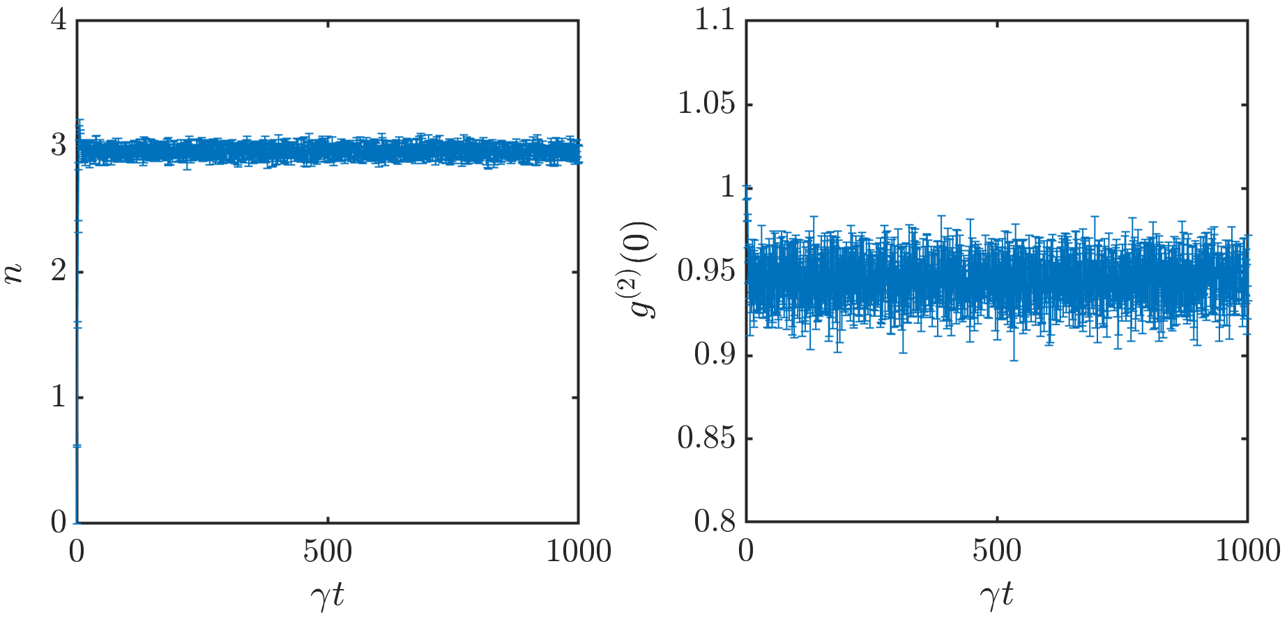
A steady state is reached quickly in this case compared to the total simulation time. One can check that the steady-state values shown here match with the values of of $n$ and $g^{(2)}(0)$ time averaged over the steady state generated by the DDBH1PP_tAv script, stored in the output file as n_Av and g2, respectively.

Excersises

• The positive-P method provides exact values of quantum observables in the limit of averaging over sufficiently many stochastic trajectories, but is limited by a noise self-amplification instability that can occur when the growth of noise, generated by interactions $U$, is not sufficiently suppressed by the dissipation $\gamma$. Try running DDBH_1site_PP for increasing values of $U$ or $F$ until trajectories start becoming unstable. Instabilities should be signalled by a message “Halt_Non_finite” in the output of the trajectory generating code, and by NaN values for observables calculated in Matlab.
• At roughly what value of $U$ do positive-P simulations become unstable for $F=\gamma$, $\Delta=0$?
• At roughly what value of $F$ do positive-P simulations become unstable for $U = 0.1\gamma$, $\Delta=0$?

1D chains

We will now look at simulating many site DDBH lattices. As the simplest example, we will focus in this tutorial on 1D chains. However, template simulation directories and Matlab post-processing scripts for simulations of 2D square lattices, and both quasi-1D and 2D Lieb lattices are also provided in our code base. We will also use this section of the tutorial to show how some of the structures in the xmds script can be used to include different boundary conditions and spatially non-uniform driving in the simulations.

We will consider a chain of 5 sites with open boundaries and driving only on the first site. Make a copy of the DDBH_Nsite_PP_template directory. We will edit some elements in the xmds script to produce the desired boundary conditions and non-uniform driving. The “hoppings” vector element is provided so that the inter-site hopping in the chain may be initialised to be arbitrarily nonuniform. The code is set up to allow for periodic boundary conditions; to change this to open boundaries, we will simply set the hopping terms between site 1 and site N (the final site) to 0 as follows:

<!--- %% Hopping coefficients j -> j+1 and j -> j-1 for each site,
      can also be used to define boundary conditions.  All = Jhop means uniform hopping on ring (periodic boundaries) -->
<vector name="hoppings" type="complex" dimensions="j">
    <components>
      J_hop_plus J_hop_minus
    </components>
    <initialisation>
      <![CDATA[
        J_hop_plus = Jhop;
        J_hop_minus = Jhop;
        J_hop_plus(j => N) = 0;
        J_hop_minus(j => 1) = 0;
       ]]>
    </initialisation>
  </vector>

The driving can be similarly set up to be nonuniform through the initialisation of the vector element “pump”. By default it is set to be uniform on all sites; to set it to only take the value given by the parameter $F$ on site 1 and be 0 otherwise, change the initialisation so it reads as follows:

<!-- Pumping, allowing for spatially non-uniform drive.  Default set to uniform all F = FPmp -->
<vector name="pump" type="complex" dimensions="j">
    <components>
      F
    </components>
    <initialisation>
      <![CDATA[
        F(j => 1) = FPmp;
       ]]>
    </initialisation>
  </vector>

Note that in xmds, any vector components not addressed explicitly in the initialisation element are set to 0 by default. Again use

xmds2 DDBH_Nsite_PP.xmds

to compile the xmds script with the changes. We will set the system size and other physical parameters via the bash runscript. Set the parameters in DDBH_Nsite_PP_runscript.sh as follows:

# Parameters; gamma = 1 taken as energy unit by default.  
N=5; # Number of sites 
Delta=0.0; # On-site energy detuning
Uint=0.1; # Two-particle interaction strength
FPmp=3.0; # Coherent drive amplitude
Jhop=3.0; # Hopping strength
time_run=1000; # end time of simulation

then use the command

./DDBH_Nsite_PP_runscript.sh

to run the simulation code and generate stochastic trajectories.

To run the Matlab analysis to generate observables, first edit analysis.m to make sure it has the correct parameters:

%Input system parameters
N = 5; % Number of sites
Delta = 0.0; % On-site energy detuning
U = 0.1; % Interaction
F = 3.0; % Coherent drive
J = 3.0; % Hopping
tf = 1000; % Final time

then on the list of scripts to run at the end, we want

%List of scripts to process data
DDBHNPP_tAv

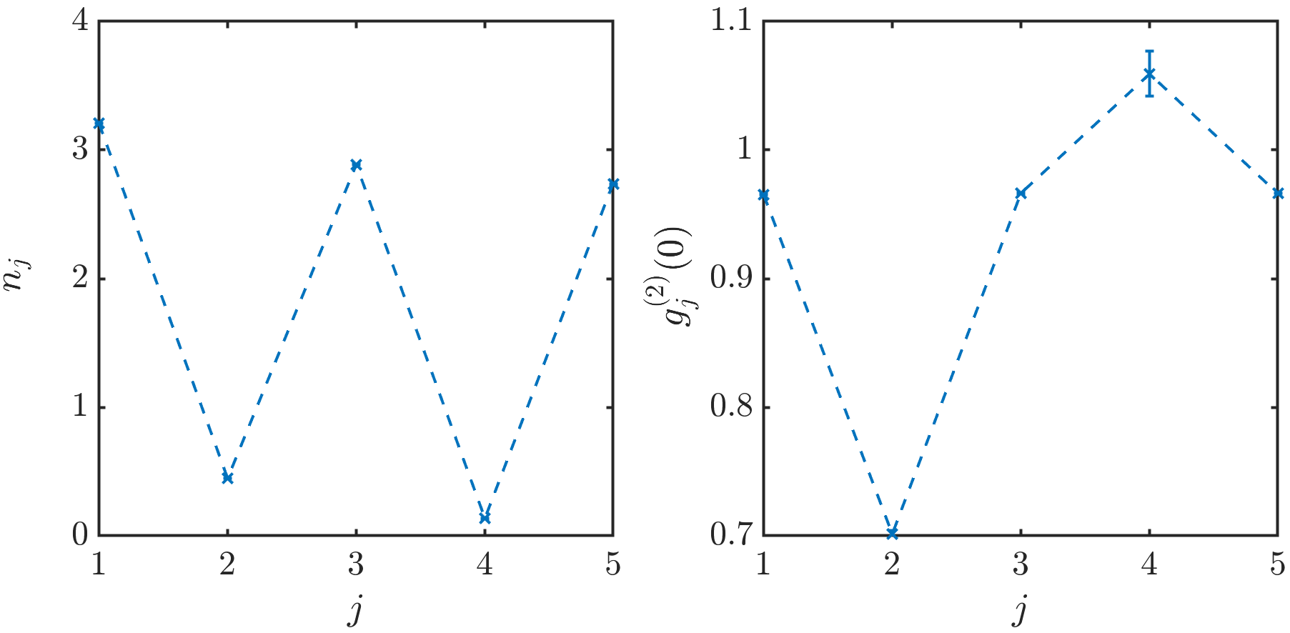
The analysis.m script can then be run in the simulation directory. The script DDBHNPP_tAv.m is set up to calculate observables including time averaging (i.e. in principle over the steady state, initial time set manually in the script) in the stochastic averaging process but keep the results separate for each site in the chain. The observables will be stored as nj for $n$ and g2j for $g^{(2)}(0)$ in the output file. After loading the output data, we can plot $n$ and $g^{(2)}(0)$ across the chain using

figure
errorbar(1:5, nj, err_nj)
figure
errorbar(1:5, g2j, err_g2j)

Subject to formatting choices, the output should look something like this:

Excersises

• A major advantage of the positive-P method is how easily it can be scaled to much larger system sizes that considered above (100s or 1000s of sites pose no issue). Set up the DDBH_Nsite_PP.xmds code so that it has open boundary conditions but uniform driving. Look how the spatially resolved $n$ and $g^{(2)}(0)$ behave for increasingly large system sizes: e.g. $N = 5, 10, 30, 50, 100, 300, 500, 1000$.
• Does the behaviour far from the edges of the chain become approximately uniform above a certain system size?
• How many sites do edge effects extend into the chain?
• How does this vary when changing $J$?